4 Time Series Regression (e.g. ECM)

4.1 Stationeritas

Show the code

library(dynlm) #for the `dynlm()` function
library(orcutt) # for the `cochrane.orcutt()` function
library(nlWaldTest) # for the `nlWaldtest()` function
library(zoo) # for time series functions (not much used here)
library(pdfetch) # for retrieving data (just mentioned here)
library(lmtest) #for `coeftest()` and `bptest()`.
library(broom) #for `glance(`) and `tidy()`
library(PoEdata) #for PoE4 datasets
library(car) #for `hccm()` robust standard errors
library(sandwich)
library(knitr) #for kable()
library(forecast)
library(dplyr)

Time Series Data adalah data beberapa variabel pada suatu unit pengamatan (seperti individu, negara, atau perusahaan) ketika pengamatan mencakup beberapa periode. Korelasi antara pengamatan selanjutnya, pentingnya tatanan dalam data dan dinamika (nilai data masa lalu mempengaruhi nilai masa kini dan masa depan) merupakan fitur time series data yang tidak terjadi dalam data cross-sectional.

Model Time Series mengasumsikan, selain asumsi regresi linier biasa, bahwa series-series data tersebut stasioner, yaitu distribusi error, serta korelasi antar error dalam beberapa periode adalah konstan sepanjang waktu. Distribusi yang konstan mensyaratkan, khususnya, bahwa variabel tersebut tidak menampilkan tren dalam mean atau variansnya; korelasi konstan menyiratkan tidak adanya pengelompokan pengamatan dalam periode tertentu.

Contoh Model Time Series:

Stationer, e.g: Regresi OLS, AutoRegressive Distributed Lag Model (ARDL), etc
Tidak Stasioner, e.g: Error Correction Models (ECM)

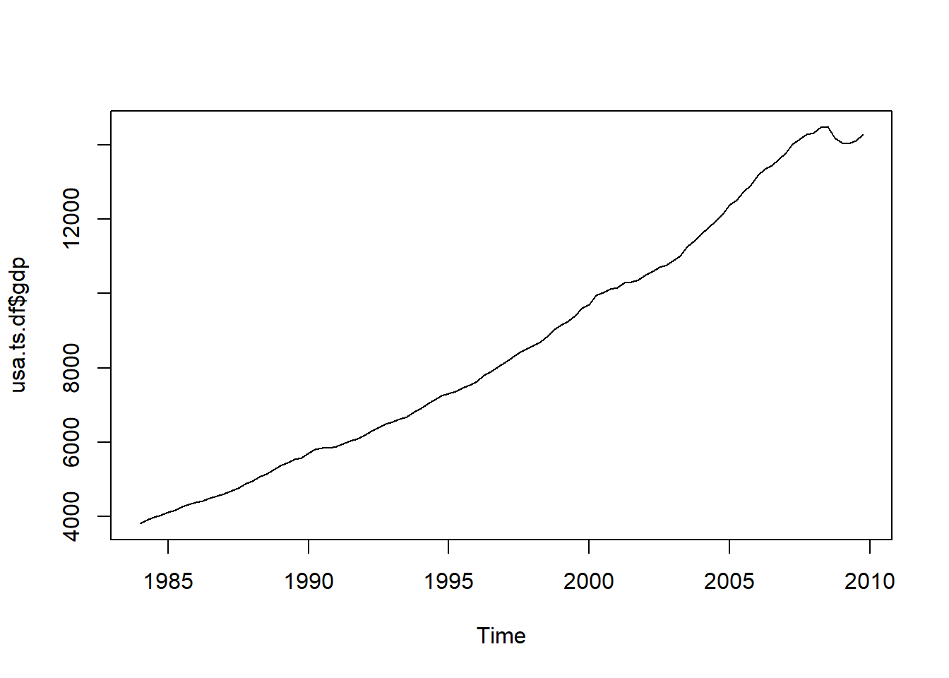
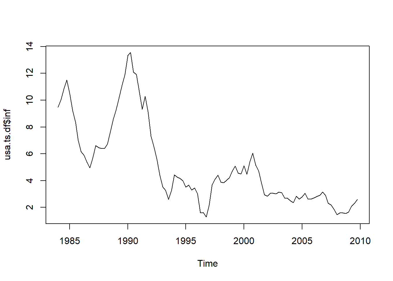
Deret waktu dikatakan nonstasioner jika distribusinya, khususnya mean, varians, atau kovarians berdasarkan waktu berubah seiring waktu. Deret waktu nonstasioner tidak dapat digunakan dalam model regresi karena dapat menimbulkan regresi palsu , yaitu hubungan yang salah karena, misalnya, tren umum pada variabel yang tidak terkait. Dua atau lebih rangkaian nonstasioner masih dapat menjadi bagian dari model regresi jika keduanya terkointegrasi, yaitu keduanya berada dalam hubungan yang stasioner.

Show the code

data("usa", package="PoEdata")
usa.ts <- ts(usa, start=c(1984,1), end=c(2009,4),
               frequency=4)
Dgdp <- diff(usa.ts[,1])
Dinf <- diff(usa.ts[,"inf"])
Df <- diff(usa.ts[,"f"])
Db <- diff(usa.ts[,"b"])
usa.ts.df <- ts.union(gdp=usa.ts[,1], # package tseries
                      inf=usa.ts[,2], 
                      f=usa.ts[,3],
                      b=usa.ts[,4],
                      Dgdp,Dinf,Df,Db,
                      dframe=TRUE)
                      
plot(usa.ts.df$gdp)

Show the code

plot(usa.ts.df$Dgdp)

Show the code

plot(usa.ts.df$inf)

Show the code

plot(usa.ts.df$Dinf)

Show the code

plot(usa.ts.df$f)

Show the code

plot(usa.ts.df$Df)

Show the code

plot(usa.ts.df$b)

Show the code

plot(usa.ts.df$Db)

Contoh Dataset:

Show the code

kable(head(usa.ts.df), 
caption="Time series data frame constructed with 'ts.union'")

Time series data frame constructed with ‘ts.union’
gdp	inf	f	b	Dgdp	Dinf	Df	Db
3807.4	9.47	9.69	11.19	NA	NA	NA	NA
3906.3	10.03	10.56	12.64	98.9	0.56	0.87	1.45
3976.0	10.83	11.39	12.64	69.7	0.80	0.83	0.00
4034.0	11.51	9.27	11.10	58.0	0.68	-2.12	-1.54
4117.2	10.51	8.48	10.68	83.2	-1.00	-0.79	-0.42
4175.7	9.24	7.92	9.76	58.5	-1.27	-0.56	-0.92

4.2 Uji Unit Root untuk Stasioneritas

4.2.1 AR1, Model Autoregressive Orde Pertama

Spesifikasi Model \[y_t=\rho y_{t-1}+v_t, |\rho|<1\]

Uji Dickey-Fuller untuk stasioneritas didasarkan pada proses AR(1) sebagaimana didefinisikan dalam Persamaan di atas.

\[H_0: \rho=1, H_1:\rho<1 \text{ (Variabel Stasioner})\]

Show the code

plot(usa.ts.df$f)

Show the code

Acf(usa.ts.df$f)

4.2.2 ADF Test USA Funds

Show the code

tseries::adf.test(usa.ts.df$f, k = 10)


    Augmented Dickey-Fuller Test

data:  usa.ts.df$f
Dickey-Fuller = -3.3726, Lag order = 10, p-value = 0.06283
alternative hypothesis: stationary

4.2.3 ADF Test USA Bonds

Show the code

plot(usa.ts.df$b)

Show the code

acf(usa.ts.df$b)

Show the code

tseries::adf.test(usa.ts.df$b, k=10)


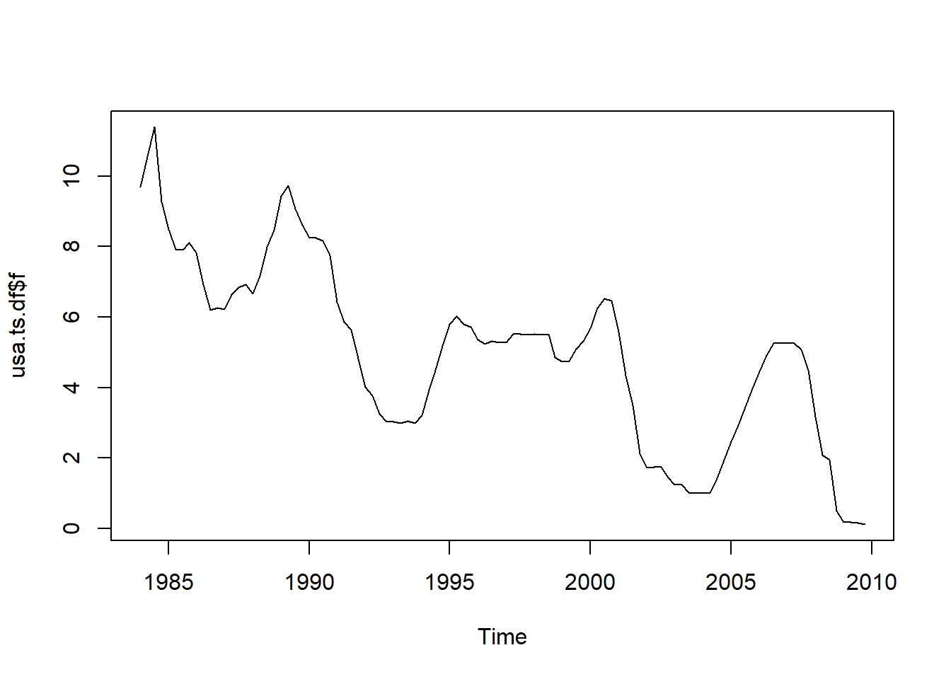
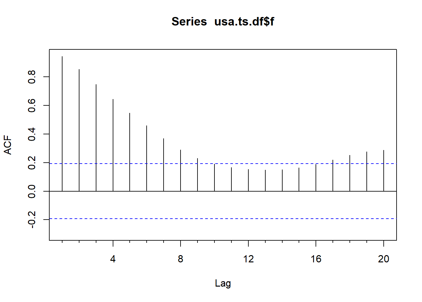
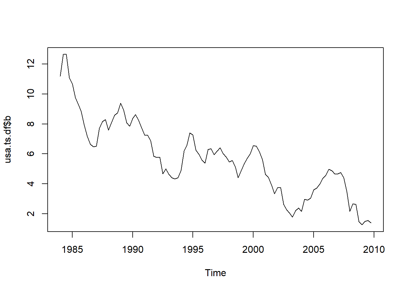
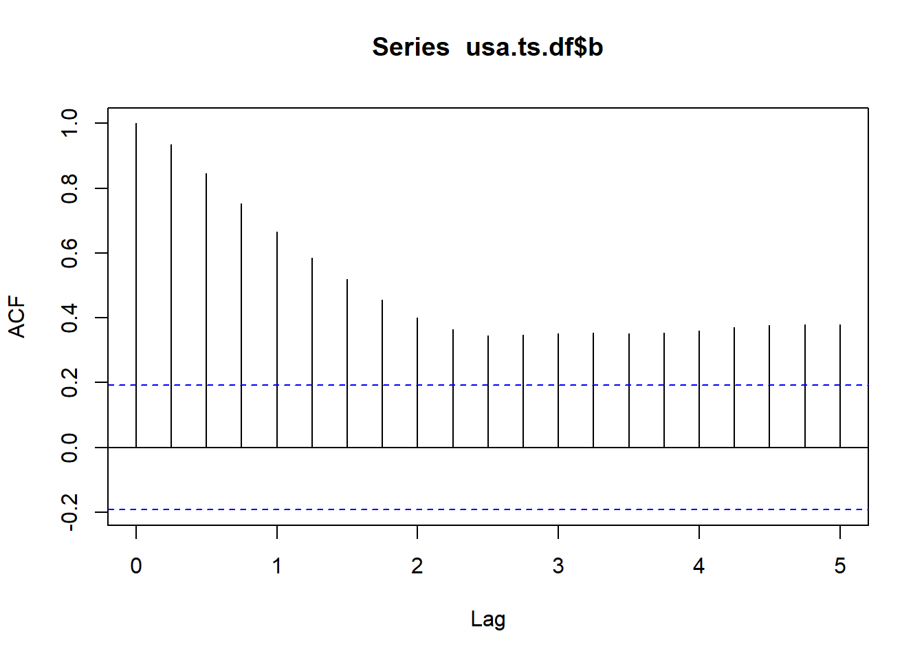
    Augmented Dickey-Fuller Test

data:  usa.ts.df$b
Dickey-Fuller = -2.9838, Lag order = 10, p-value = 0.1687
alternative hypothesis: stationary

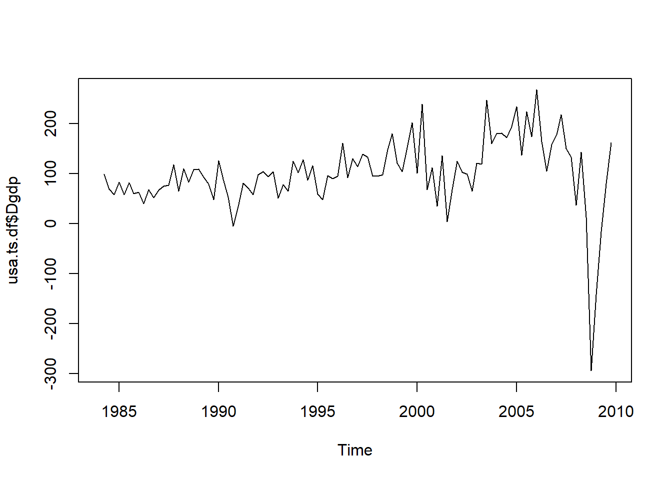
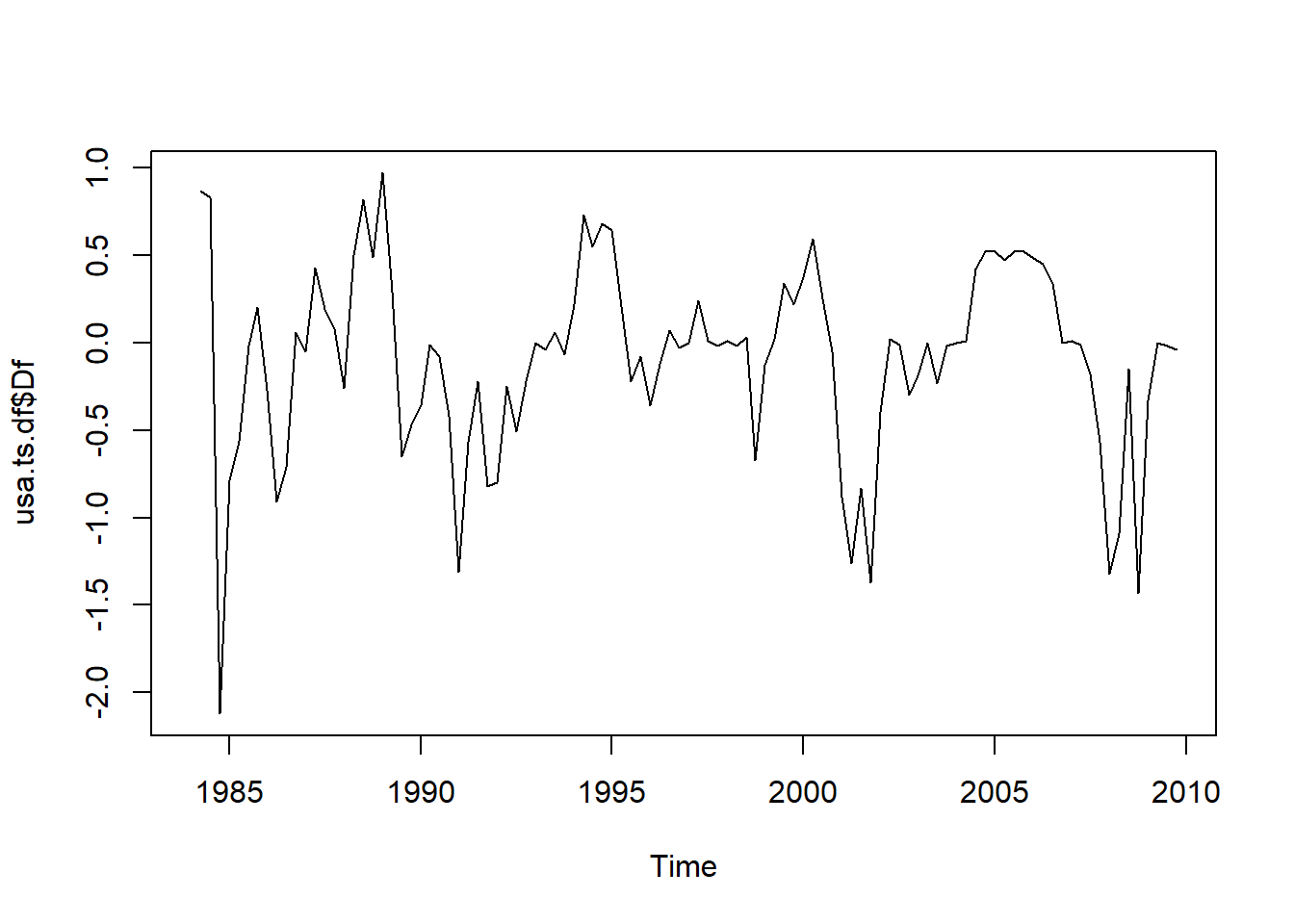
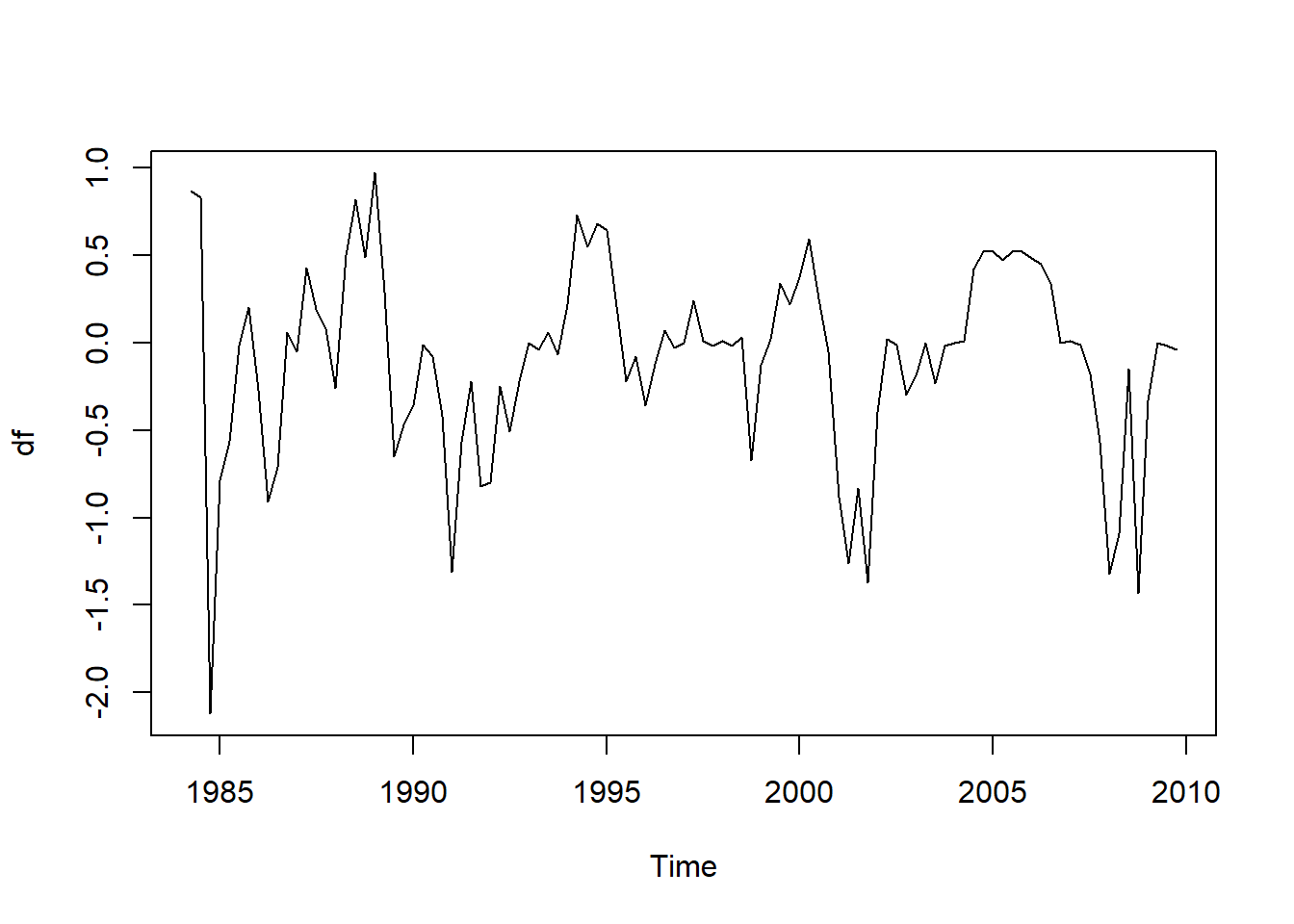
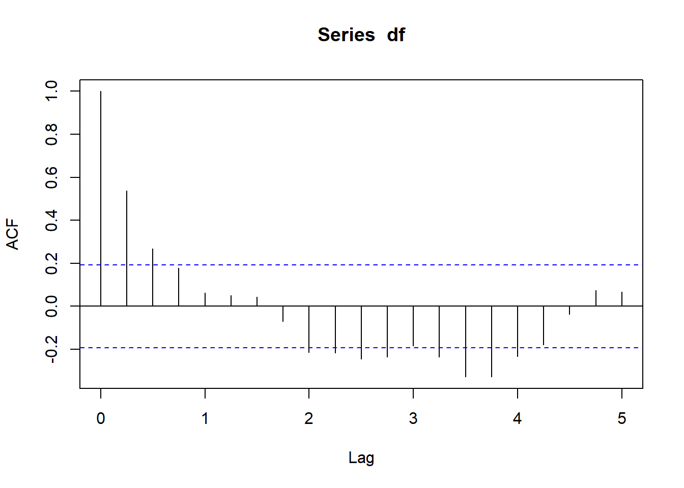
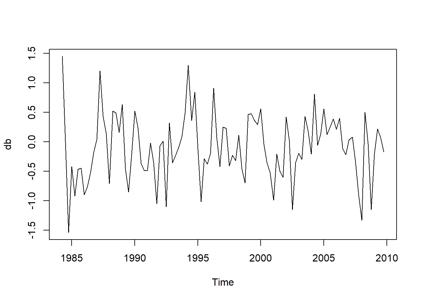
4.3 Differensiasi

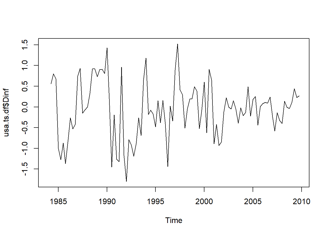
Konsep yang erat kaitannya dengan stasioneritas adalah orde integrasi, yaitu berapa kali kita perlu mendiferensiasikan suatu deret hingga deret tersebut stasioner.

I(0) - stasioner dalam level
I(1) jika deret tersebut tidak stasioner pada tingkat-tingkatnya, tetapi stasioner pada perbedaan pertamanya.

Show the code

df <- diff(usa.ts.df$f)
plot(df)

Show the code

acf(df)

Show the code

tseries::adf.test(df, k=2)


    Augmented Dickey-Fuller Test

data:  df
Dickey-Fuller = -4.1782, Lag order = 2, p-value = 0.01
alternative hypothesis: stationary

Show the code

db <- diff(usa.ts.df$b)
plot(db)

Show the code

acf(db)

Show the code

tseries::adf.test(db, k=2)


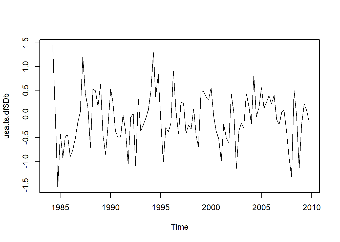
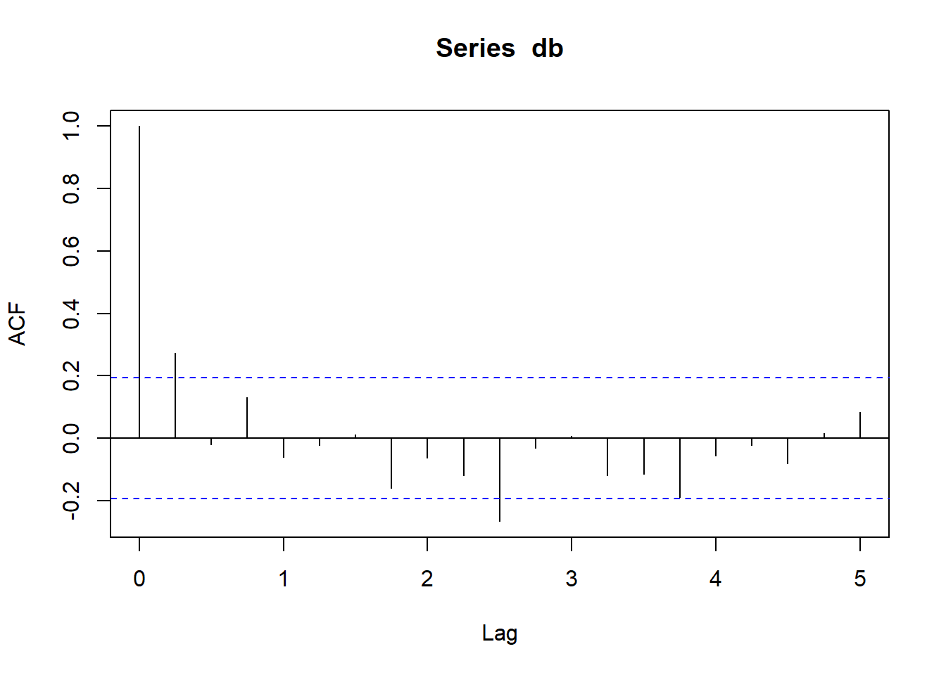
    Augmented Dickey-Fuller Test

data:  db
Dickey-Fuller = -4.3976, Lag order = 2, p-value = 0.01
alternative hypothesis: stationary

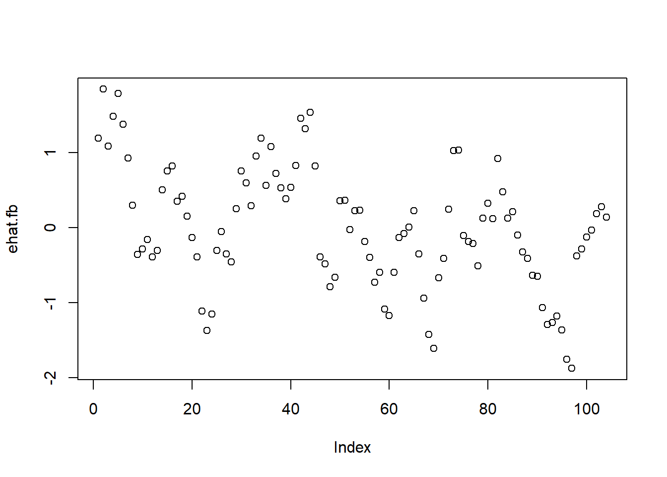
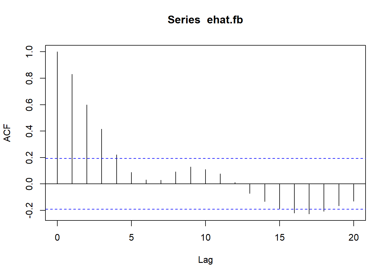
4.4 Kointegrasi

Dua seri terkointegrasi ketika trennya tidak berbeda jauh dan dalam beberapa hal serupa. Uji kointegrasi pada kenyataannya adalah uji stasioneritas Dickey-Fuler terhadap residu, dan hipotesis nolnya adalah nonkointegrasi. Dengan kata lain, kita ingin menolak hipotesis nol dalam uji kointegrasi, seperti yang kita inginkan dalam uji stasioneritas.

Mari kita terapkan metode ini untuk menentukan keadaan kointegrasi antara rangkaian dan dalam kumpulan data

Show the code

fb.dyn <- dynlm(b~f, data = usa)
ehat.fb <- resid(fb.dyn)
summary(fb.dyn)


Time series regression with "numeric" data:
Start = 1, End = 104

Call:
dynlm(formula = b ~ f, data = usa)

Residuals:
    Min      1Q  Median      3Q     Max 
-1.8777 -0.4220 -0.0445  0.5062  1.8440 

Coefficients:
            Estimate Std. Error t value Pr(>|t|)    
(Intercept)  1.13983    0.17408   6.548  2.4e-09 ***
f            0.91441    0.03108  29.421  < 2e-16 ***
---
Signif. codes:  0 '***' 0.001 '**' 0.01 '*' 0.05 '.' 0.1 ' ' 1

Residual standard error: 0.8102 on 102 degrees of freedom
Multiple R-squared:  0.8946,    Adjusted R-squared:  0.8936 
F-statistic: 865.6 on 1 and 102 DF,  p-value: < 2.2e-16

Show the code

#db <- diff(usa.ts.df$b)
plot(ehat.fb)

Show the code

acf(ehat.fb)

Show the code

tseries::adf.test(ehat.fb, k=4)


    Augmented Dickey-Fuller Test

data:  ehat.fb
Dickey-Fuller = -4.0009, Lag order = 4, p-value = 0.01184
alternative hypothesis: stationary

Show the code

b=usa.ts.df$b
f=usa.ts.df$f
bfx <- as.matrix(cbind(b,f), demean=FALSE)
tseries::po.test(bfx)


    Phillips-Ouliaris Cointegration Test

data:  bfx
Phillips-Ouliaris demeaned = -20.508, Truncation lag parameter = 1,
p-value = 0.04986

4.5 Error Correction Model (ECM)

An Error Correction Model (ECM) merupakan metode standard untuk memodelkan data time series.
The ECM makes it possible to deal with nonstationary data series and separates the long and short run.

4.5.1 Two Steps Engle Granger

Spesifikasi Model

Tahap 1

\[y_t =\beta_0+\beta_1 x_t+u_t \]

\[\hat{u_t}=y_t -\hat\beta_0-\hat\beta_1 x_t\]

Dimana:

\(\beta_1\) merupakan Koefisien Model Long-run

Tahap 2

\[\Delta y_t=\beta_2+\beta_3 \Delta x_t - \pi_1 \hat u_{t-1}+\varepsilon_t \]

Dimana:

\(\pi_1\) is the feedback effect, or the adjustment effect, or error correction coefficient and shows how much of the disequilibrium is being corrected.
\(\varepsilon_t\) merupakan white noise error term

** Step 1 **

Show the code

b=usa.ts.df$b
f=usa.ts.df$f
fb.dyn <- dynlm(b~f)
summary(fb.dyn)


Time series regression with "ts" data:
Start = 1984(1), End = 2009(4)

Call:
dynlm(formula = b ~ f)

Residuals:
    Min      1Q  Median      3Q     Max 
-1.8777 -0.4220 -0.0445  0.5062  1.8440 

Coefficients:
            Estimate Std. Error t value Pr(>|t|)    
(Intercept)  1.13983    0.17408   6.548  2.4e-09 ***
f            0.91441    0.03108  29.421  < 2e-16 ***
---
Signif. codes:  0 '***' 0.001 '**' 0.01 '*' 0.05 '.' 0.1 ' ' 1

Residual standard error: 0.8102 on 102 degrees of freedom
Multiple R-squared:  0.8946,    Adjusted R-squared:  0.8936 
F-statistic: 865.6 on 1 and 102 DF,  p-value: < 2.2e-16

Show the code

ect=fb.dyn$residuals
tseries::adf.test(ect)


    Augmented Dickey-Fuller Test

data:  ect
Dickey-Fuller = -4.0009, Lag order = 4, p-value = 0.01184
alternative hypothesis: stationary

Signifikansi Menunjukkan adanya kointegrasi

** Step 2 **

Show the code

# Set ECT dan Variabel penting lainnya menjadi time Series
ect=ts(ect,start=c(1984,1), end=c(2009,4),
               frequency=4)
ect1=ts(ect,start=c(1984,2), end=c(2009,4),
               frequency=4)

b=ts(b,start=c(1984,1), end=c(2009,4),
               frequency=4)

f=ts(f,start=c(1984,1), end=c(2009,4),
               frequency=4)

L1.b=stats::lag(b,-1)
L1.f=stats::lag(f,-1)
L1.b=ts(L1.b,start=c(1984,2), end=c(2009,4),
               frequency=4)
L1.f=ts(L1.f,start=c(1984,2), end=c(2009,4),
               frequency=4)

tsdata=ts.union(b,f,L1.b,L1.f,ect,ect1)
head(tsdata)

            b     f  L1.b  L1.f      ect     ect1
1984 Q1 11.19  9.69    NA    NA 1.189524       NA
1984 Q2 12.64 10.56 11.19  9.69 1.843986 1.189524
1984 Q3 12.64 11.39 12.64 10.56 1.085025 1.843986
1984 Q4 11.10  9.27 12.64 11.39 1.483577 1.085025
1985 Q1 10.68  8.48 11.10  9.27 1.785962 1.483577
1985 Q2  9.76  7.92 10.68  8.48 1.378032 1.785962

Show the code

regECM1=lm(diff(b)~diff(f)+ect1)
summary(regECM1)


Call:
lm(formula = diff(b) ~ diff(f) + ect1)

Residuals:
     Min       1Q   Median       3Q      Max 
-1.03574 -0.30858 -0.03668  0.24341  1.06092 

Coefficients:
            Estimate Std. Error t value Pr(>|t|)    
(Intercept) -0.03039    0.04265  -0.713   0.4778    
diff(f)      0.69873    0.08128   8.597 1.16e-13 ***
ect1        -0.12307    0.05502  -2.237   0.0275 *  
---
Signif. codes:  0 '***' 0.001 '**' 0.01 '*' 0.05 '.' 0.1 ' ' 1

Residual standard error: 0.4261 on 100 degrees of freedom
Multiple R-squared:  0.426, Adjusted R-squared:  0.4145 
F-statistic: 37.11 on 2 and 100 DF,  p-value: 8.811e-13

4.5.2 One Step ECM

\[\Delta y_t=\beta_2+\beta_3 \Delta x_t - \pi_1 \hat u_{t-1}+\varepsilon_t \] \[\Delta y_t=\beta_2+\beta_3 \Delta x_t - \pi_1(y_{t-1} -\hat\beta_0-\hat\beta_1 x_{t-1})+\varepsilon_t \]

\[\Delta y_t=\beta_2+\beta_3 \Delta x_t - \pi_1(y_{t-1} -\hat\beta_0-\hat\beta_1 x_{t-1})+\varepsilon_t \]

\[\Delta y_t=\beta_2+\beta_3 \Delta x_t - \pi_1y_{t-1} + \pi_1\hat\beta_0+ \pi_1\hat\beta_1 x_{t-1}+\varepsilon_t\]

Susun kembali, dan misalkan jika \(\pi_1=-\alpha_1\) dan \(\pi_1\beta_1=\alpha_2\)

\[\Delta y_t=\alpha_0 + \alpha_1 y_{t-1} + \alpha_2 x_{t-1}+\alpha_3 \Delta x_t+\varepsilon_t\]

Maka diperoleh hubungan

\[\Delta y_t=\alpha_0 - \alpha_1 (y_{t-1} + \frac{\alpha_2}{\alpha_1} x_{t-1})+\alpha_3 \Delta x_t+\varepsilon_t\]

Long-Run Coefficient Model \[\hat \beta_1=-\frac{\alpha_2}{\alpha_1} \]

Show the code

regECM2=lm(diff(b)~L1.b+L1.f+diff(f))
summary(regECM2)


Call:
lm(formula = diff(b) ~ L1.b + L1.f + diff(f))

Residuals:
     Min       1Q   Median       3Q      Max 
-1.06697 -0.30745 -0.05507  0.26760  1.13987 

Coefficients:
            Estimate Std. Error t value Pr(>|t|)    
(Intercept)  0.22636    0.11166   2.027   0.0453 *  
L1.b        -0.12001    0.05476  -2.191   0.0308 *  
L1.f         0.08565    0.05338   1.605   0.1118    
diff(f)      0.68582    0.08133   8.433 2.82e-13 ***
---
Signif. codes:  0 '***' 0.001 '**' 0.01 '*' 0.05 '.' 0.1 ' ' 1

Residual standard error: 0.4238 on 99 degrees of freedom
Multiple R-squared:  0.4379,    Adjusted R-squared:  0.4209 
F-statistic: 25.71 on 3 and 99 DF,  p-value: 2.214e-12

Show the code

# Homoskedastisitas Check
library(car)
ncvTest(regECM2)

Non-constant Variance Score Test 
Variance formula: ~ fitted.values 
Chisquare = 0.000515675, Df = 1, p = 0.98188

Show the code

# Homoskedastisitas Check
library(lmtest)
bgtest(regECM2)


    Breusch-Godfrey test for serial correlation of order up to 1

data:  regECM2
LM test = 2.2827, df = 1, p-value = 0.1308

4.5.3 ARDL

Show the code

library(ARDL)
ardl1=ardl(b~f, data=usa.ts.df, order=c(1,1))
summary(ardl1)


Time series regression with "ts" data:
Start = 2, End = 104

Call:
dynlm::dynlm(formula = full_formula, data = data, start = start, 
    end = end)

Residuals:
     Min       1Q   Median       3Q      Max 
-1.06697 -0.30745 -0.05507  0.26760  1.13987 

Coefficients:
            Estimate Std. Error t value Pr(>|t|)    
(Intercept)  0.22636    0.11166   2.027   0.0453 *  
L(b, 1)      0.87999    0.05476  16.070  < 2e-16 ***
f            0.68582    0.08133   8.433 2.82e-13 ***
L(f, 1)     -0.60017    0.08077  -7.431 3.89e-11 ***
---
Signif. codes:  0 '***' 0.001 '**' 0.01 '*' 0.05 '.' 0.1 ' ' 1

Residual standard error: 0.4238 on 99 degrees of freedom
Multiple R-squared:  0.9706,    Adjusted R-squared:  0.9697 
F-statistic:  1089 on 3 and 99 DF,  p-value: < 2.2e-16

Show the code

bounds_f_test(ardl1, case=3)


    Bounds F-test (Wald) for no cointegration

data:  d(b) ~ L(b, 1) + L(f, 1) + d(f)
F = 3.5753, p-value = 0.2269
alternative hypothesis: Possible cointegration
null values:
   k    T 
   1 1000

Show the code

bounds_t_test(ardl1, case=3)


    Bounds t-test for no cointegration

data:  d(b) ~ L(b, 1) + L(f, 1) + d(f)
t = -2.1915, p-value = 0.3339
alternative hypothesis: Possible cointegration
null values:
   k    T 
   1 1000

Show the code

ecm=uecm(ardl1)
summary(ecm)


Time series regression with "ts" data:
Start = 2, End = 104

Call:
dynlm::dynlm(formula = full_formula, data = data, start = start, 
    end = end)

Residuals:
     Min       1Q   Median       3Q      Max 
-1.06697 -0.30745 -0.05507  0.26760  1.13987 

Coefficients:
            Estimate Std. Error t value Pr(>|t|)    
(Intercept)  0.22636    0.11166   2.027   0.0453 *  
L(b, 1)     -0.12001    0.05476  -2.191   0.0308 *  
L(f, 1)      0.08565    0.05338   1.605   0.1118    
d(f)         0.68582    0.08133   8.433 2.82e-13 ***
---
Signif. codes:  0 '***' 0.001 '**' 0.01 '*' 0.05 '.' 0.1 ' ' 1

Residual standard error: 0.4238 on 99 degrees of freedom
Multiple R-squared:  0.4379,    Adjusted R-squared:  0.4209 
F-statistic: 25.71 on 3 and 99 DF,  p-value: 2.214e-12