Show the code
Unbalanced panel data set with 1031 rows and the following time period frequencies: 1976 1977 1978 1979 1980 1981 1982 1983 1984
80 138 140 140 140 140 140 78 35 Linear dynamic panel data models account for dynamics and unobserved individual-specific heterogeneity. Due to the presence of lagged dependent variables, applying ordinary least squares including individual-specific dummy variables is inconsistent.
\[y_{it}=\alpha y_{i,t-1}+\beta x_{i,t}+u_{i,t}\] \[u_{i,t}=\eta_i+\varepsilon_{i,t}\] \[y_{it}=\alpha y_{i,t-1}+\beta x_{i,t}+\eta_i+\varepsilon_{i,t}\]
First Difference to elliminate \(\eta_i\)
\[\Delta y_{it}=\alpha \Delta y_{i,t-1}+\beta \Delta x_{i,t}+\Delta \varepsilon_{i,t}\]
n=140 firms T=9
Unbalanced panel data set with 1031 rows and the following time period frequencies: 1976 1977 1978 1979 1980 1981 1982 1983 1984
80 138 140 140 140 140 140 78 35 strucUPD.plot(dat,i.name = "firm",t.name = "year")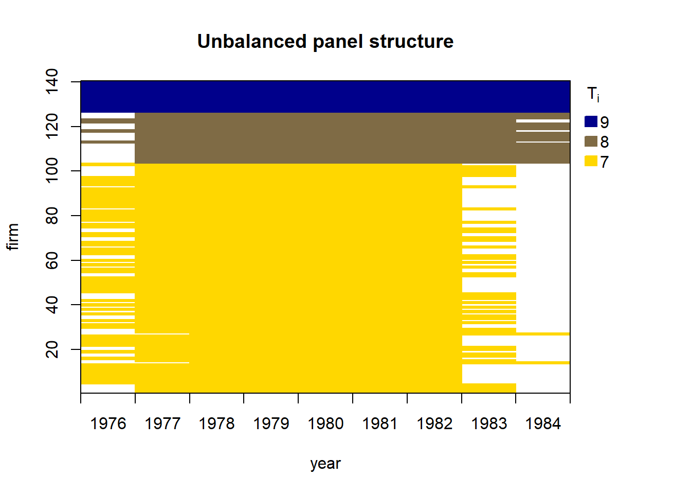
m1 <- pdynmc(
    dat = dat,
    varname.i = "firm",
    varname.t = "year",
    use.mc.diff = TRUE,
    use.mc.lev = FALSE,
    use.mc.nonlin = FALSE,
    include.y = TRUE,
    varname.y = "n",
    lagTerms.y = 2,
    fur.con = TRUE,
    fur.con.diff = TRUE,
    fur.con.lev = FALSE,
    varname.reg.fur = c("w", "k", "ys"),
    lagTerms.reg.fur = c(1,2,2),
    include.dum = TRUE,
    dum.diff = TRUE,
    dum.lev = FALSE,
    varname.dum = "year",
    w.mat = "iid.err",
    std.err = "corrected",
    estimation = "twostep",
    opt.meth = "none"
)
summary(m1)
Dynamic linear panel estimation (twostep)
GMM estimation steps: 2

Coefficients:
      Estimate Std.Err.rob z-value.rob Pr(>|z.rob|)
L1.n   0.62871     0.19341       3.251      0.00115 **
L2.n  -0.06519     0.04505      -1.447      0.14790
L0.w  -0.52576     0.15461      -3.401      0.00067 ***
L1.w   0.31129     0.20300       1.533      0.12528
L0.k   0.27836     0.07280       3.824      0.00013 ***
L1.k   0.01410     0.09246       0.152      0.87919
L2.k  -0.04025     0.04327      -0.930      0.35237
L0.ys  0.59192     0.17309       3.420      0.00063 ***
L1.ys -0.56599     0.26110      -2.168      0.03016 *
L2.ys  0.10054     0.16110       0.624      0.53263
1979   0.01122     0.01168       0.960      0.33706
1980   0.02307     0.02006       1.150      0.25014
1981  -0.02136     0.03324      -0.642      0.52087
1982  -0.03112     0.03397      -0.916      0.35967
1983  -0.01799     0.03693      -0.487      0.62626
1976  -0.02337     0.03661      -0.638      0.52347
---
Signif. codes:  0 '***' 0.001 '**' 0.01 '*' 0.05 '.' 0.1 ' ' 1

 41 total instruments are employed to estimate 16 parameters
 27 linear (DIF)
 8 further controls (DIF)
 6 time dummies (DIF)

J-Test (overid restrictions):  31.38 with 25 DF, pvalue: 0.1767
F-Statistic (slope coeff):  269.16 with 10 DF, pvalue: <0.001
F-Statistic (time dummies): 15.43 with 6 DF, pvalue: 0.0172mtest.fct(m1,t.order = 2)
    Arellano and Bond (1991) serial correlation test of degree 2

data:  2step GMM Estimation
normal = -0.36744, p-value = 0.7133
alternative hypothesis: serial correlation of order 2 in the error terms
The test does not reject the null hypothesis at any plausible significance level and provides no indication that the model specification might be inadequate.
jtest.fct(m1)
    J-Test of Hansen

data:  2step GMM Estimation
chisq = 31.381, df = 25, p-value = 0.1767
alternative hypothesis: overidentifying restrictions invalidwald.fct(m1,param = "all")
    Wald test

data:  2step GMM Estimation
chisq = 1104.7, df = 16, p-value < 2.2e-16
alternative hypothesis: at least one time dummy and/or slope coefficient is not equal to zero