2 Regresi Linear (Ordinary Least Squares)

Tahapan Regresi

Spesifikasi Model (termasuk: Identifikasi Masalah)
Pengumpulan Data
- Cross Section (Individu: n, periode: 1)
- Time Series (Individu: 1, periode: t)
- Pooled (Individu: n, periode: t)
Estimasi Parameter
Pengujian Hipotesis, Asumsi, dan Kelayakan Model
Analisis/Interpretasi/Peramalan

Show the code

# Packages Library yang digunakan
library(bookdown)
library(PoEdata)
library(knitr)
library(xtable)
library(printr)
library(stargazer)
library(rmarkdown)
library(lmtest) #for coeftest() and bptest().
library(broom) #for glance() and tidy()
library(PoEdata) #for PoE4 datasets
library(car) #for hccm() robust standard errors
library(sandwich)
library(knitr)

2.1 Spesifikasi Model Umum

Model Regresi Linier mengasumsikan bahwa terdapat hubungan linier antara variabel terikat dan variabel bebas.

\[y_i =\beta_0 +\beta_1 x_{1i}+\beta_2 x_{2i}+...+\beta_k x_{ki}+\varepsilon_i\]

Dimana:

\(y_i=\) variabel tidak bebas individu -i
\(x_{ki}=\) variabel bebas ke-k individu -i
\(\varepsilon_{i}=\) residual individu -i

2.1.1 Spesifikasi Model Regresi OLS

Linear: \(y=\beta_0+\beta_1 X\)
Semi-Log/Log-Lin: \(log(y)=\beta_0+\beta_1 X\)
Semi-Log/Lin-Log: \(log(y)=\beta_0+\beta_1 log(X)\)
Double-Log/Log-Log: \(log(y)=\beta_0+\beta_1 log(X)\)
etc

2.1.2 Spesifikasi Model Contoh: Hubungan Pendapatan terhadap Pengeluaran Makanan

Show the code

library(PoEdata)
data(food)
head(food)

food_exp	income
115.22	3.69
135.98	4.39
119.34	4.75
114.96	6.03
187.05	12.47
243.92	12.98

Data berjumlah 40 observasi. Variabel yang diamati ada 2. Data selengkapnya dapat diakses pada link yang disediakan.

Show the code

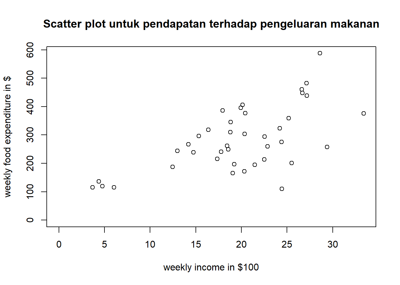
data("food", package="PoEdata")
plot(food$income, food$food_exp, 
     ylim=c(0, max(food$food_exp)),
     xlim=c(0, max(food$income)),
     xlab="weekly income in $100", 
     ylab="weekly food expenditure in $", 
     type = "p",
     main="Scatter plot untuk pendapatan terhadap pengeluaran makanan")

\[\text{Food Expenditure}_i=\beta_0+\beta_1 \text{Income}_i +\varepsilon_i\] \[\varepsilon_i \sim \text{Normal}(0,\sigma^2) \]

2.2 Estimasi Parameter dengan Regresi

Show the code

mod1 <- lm(food_exp ~ income, data = food)
b0 <- coef(mod1)[[1]]
b1 <- coef(mod1)[[2]]
smod1 <- summary(mod1)
smod1


Call:
lm(formula = food_exp ~ income, data = food)

Residuals:
     Min       1Q   Median       3Q      Max 
-223.025  -50.816   -6.324   67.879  212.044 

Coefficients:
            Estimate Std. Error t value Pr(>|t|)    
(Intercept)   83.416     43.410   1.922   0.0622 .  
income        10.210      2.093   4.877 1.95e-05 ***
---
Signif. codes:  0 '***' 0.001 '**' 0.01 '*' 0.05 '.' 0.1 ' ' 1

Residual standard error: 89.52 on 38 degrees of freedom
Multiple R-squared:  0.385, Adjusted R-squared:  0.3688 
F-statistic: 23.79 on 1 and 38 DF,  p-value: 1.946e-05

Show the code

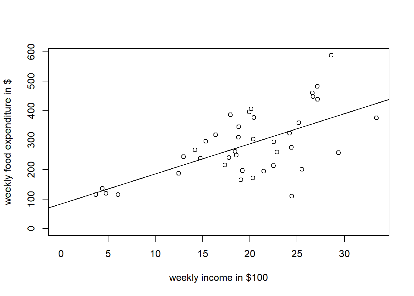
plot(food$income, food$food_exp, 
     xlab="weekly income in $100", 
     ylab="weekly food expenditure in $", 
     ylim=c(0, max(food$food_exp)),
     xlim=c(0, max(food$income)),
     type = "p")
abline(b0,b1)

2.2.1 Estimasi Selang Kepercayaan

Show the code

ci <- confint(mod1)
print(ci)

                2.5 %    97.5 %
(Intercept) -4.463279 171.29528
income       5.972052  14.44723

2.3 Pengujian Hipotesis, Asumsi, dan Kelayakan Model

2.3.1 Overall Test

Gunakan p value dari F-Statistik

\(H_0 :\) Tidak ada variabel yang signifikan dalam model

\(H_1 :\) Minimal ada 1 variabel yang signifikan dalam model

\(\alpha=0.05\)

Keputusan: Tolak \(H_0\), karena \(p-value <\alpha\)

Kesimpulan: Dengan tingkat keyakinan 95%, cukup bukti untuk menyatakan bahwa minimal ada 1 variabel yang signifikan dalam model.

2.3.2 Partial Test

Gunakan p value dari t-Statistik

\(H_0 : \beta_1=0\) variabel tidak signifikan dalam model

\(H_1 : \beta_1 \neq 0\) variabel signifikan dalam model

\(\alpha=0.05\)

Statistik Uji: \[t=\frac{\hat{\beta_1}-\beta_1}{se(\hat{\beta_1})}\]

Keputusan: Tolak \(H_0\), karena \(p-value <\alpha\)

Kesimpulan: Dengan tingkat keyakinan 95%, cukup bukti untuk menyatakan bahwa variabel signifikan dalam model.

2.3.3 Pengecekan Asumsi/Diagnosa Residual-Residual Diagnostic

2.3.3.1 Linearitas

2.3.3.2 Independensi

2.3.3.3 Normalitas

Show the code

hist(mod1$residuals)

2.3.3.4 Homoskedastisitas

Show the code

plot(mod1)

2.3.4 Kelayakan Model

Substansi
Statistik, contohnya: \((R^2)\)

2.3.4.1 Koefisien Determinasi (\(R^2\))

\[SST=SSR+SSE\]

Show the code

anova1=anova(mod1)
anova1

	Df	Sum Sq	Mean Sq	F value	Pr(>F)
income	1	190627.0	190626.984	23.78884	1.95e-05
Residuals	38	304505.2	8013.294	NA	NA

Show the code

r2=anova1$"Sum Sq"[1]/sum(anova1$"Sum Sq")

\(SST\) = 4.951322^{5}

\(R^2\) = 0.385

Artinya: 38.5 % proporsi variasi y yang dapat dijelaskan oleh model/variabel x.

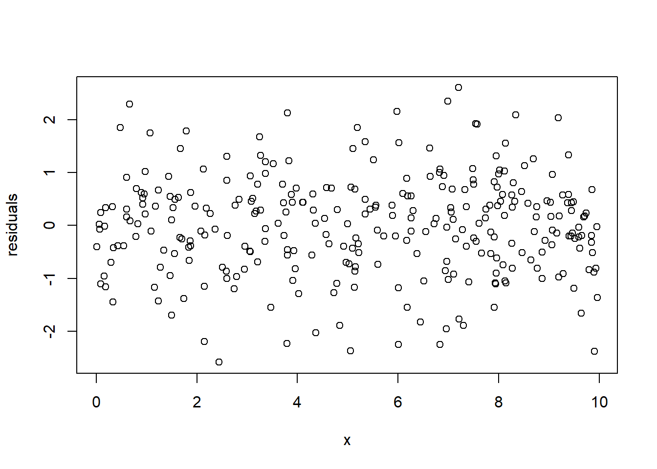
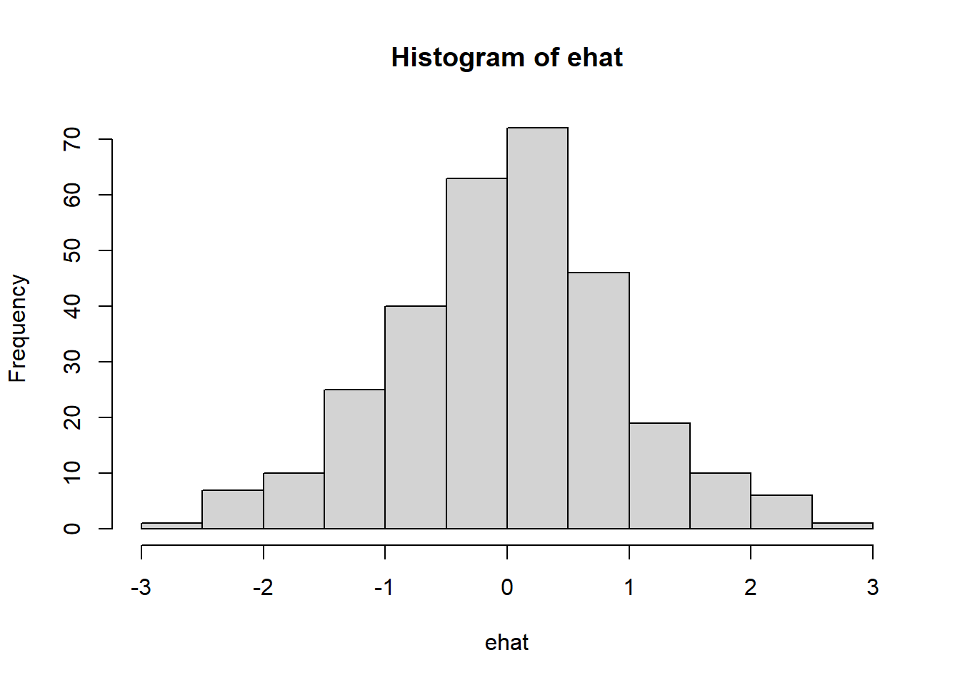
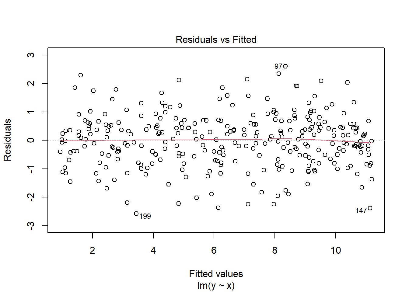
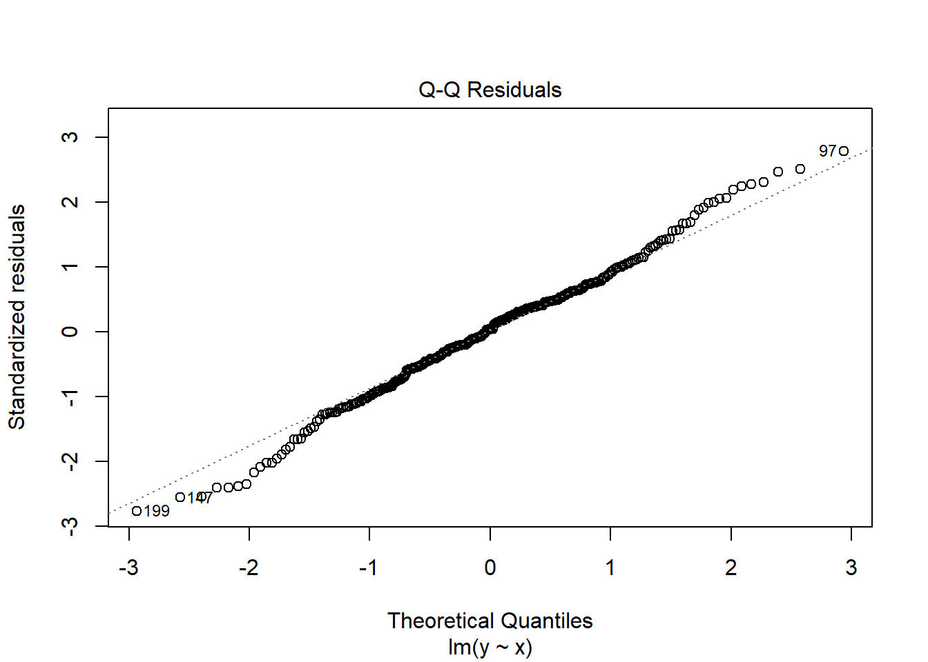
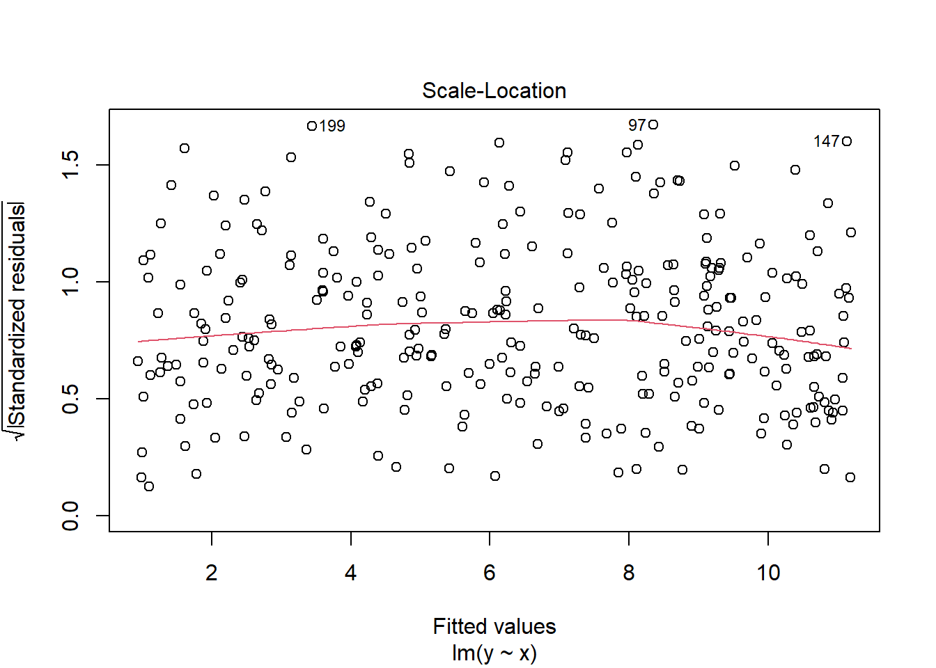
2.3.5 Contoh Pengecekan Asumsi yang sesuai/Ideal

Show the code

set.seed(12345)   #sets the seed for the random number generator
x <- runif(300, 0, 10)
e <- rnorm(300, 0, 1)
y <- 1+x+e
mod3 <- lm(y~x)
ehat <- resid(mod3)
plot(x,ehat, xlab="x", ylab="residuals")

Show the code

hist(ehat)

Show the code

plot(mod3)

2.4 Analisis/Interpretasi/Peramalan

2.4.1 Peramalan

Show the code

newx <- data.frame(income = c(20, 25, 27))
yhat <- predict(mod1, newx)
names(yhat) <- c("income=$2000", "$2500", "$2700") 
yhat  # prints the result

income=$2000        $2500        $2700 
    287.6089     338.6571     359.0764

2.4.2 Interpretasi

Show the code

mod1


Call:
lm(formula = food_exp ~ income, data = food)

Coefficients:
(Intercept)       income  
      83.42        10.21

Hati-hati menginterpretasikan Estimasi \(\beta_0\)
Interpretasi dari Estimasi \(\beta_1\)

Setiap Terjadi Kenaikan Income sebesar USD 100 (Kenaikannya sebesar 1 satuan, tetapi satuan x dalam hal ini income adalah USD 100), terjadi kenaikan pengeluaran makanan sebesar USD 10,21 (satuan y dalam hal ini adalah USD).

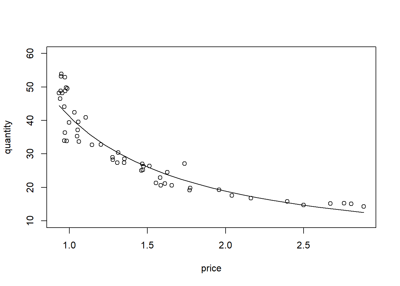
Extras: Model Log-log

Show the code

# Calculating log-log demand for chicken
data("newbroiler", package="PoEdata")
mod6 <- lm(log(q)~log(p), data=newbroiler)
b1 <- coef(mod6)[[1]]
b2 <- coef(mod6)[[2]]
smod6 <- summary(mod6)
tbl <- data.frame(xtable(smod6))
kable(tbl, caption="Model Hubungan Harga terhadap Permintaan Ayam")

Model Hubungan Harga terhadap Permintaan Ayam
	Estimate	Std..Error	t.value	Pr…t..
(Intercept)	3.716944	0.0223594	166.23619	0
log(p)	-1.121358	0.0487564	-22.99918	0

Show the code

# Drawing the fitted values of the log-log equation
ngrid <- 20 # number of drawing points 
xmin <- min(newbroiler$p)
xmax <- max(newbroiler$p)
step <- (xmax-xmin)/ngrid # grid dimension
xp <- seq(xmin, xmax, step)
predicty=exp(b1+b2*log(xp))
plot(newbroiler$p, newbroiler$q, ylim=c(10,60),
     xlab="price", ylab="quantity")
lines(predicty~xp, lty=1, col="black")

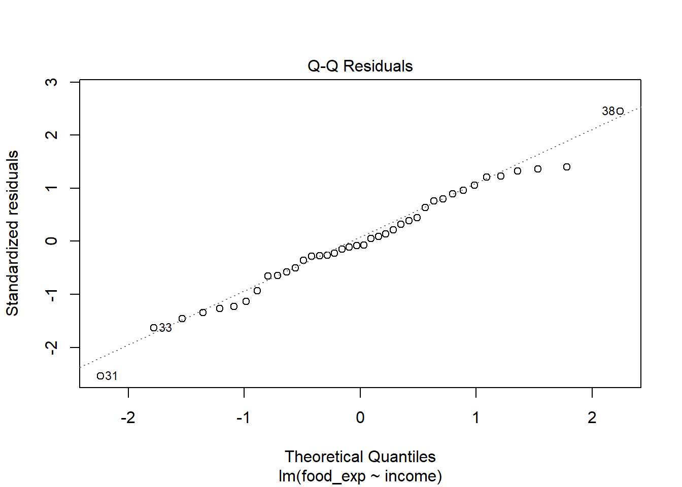
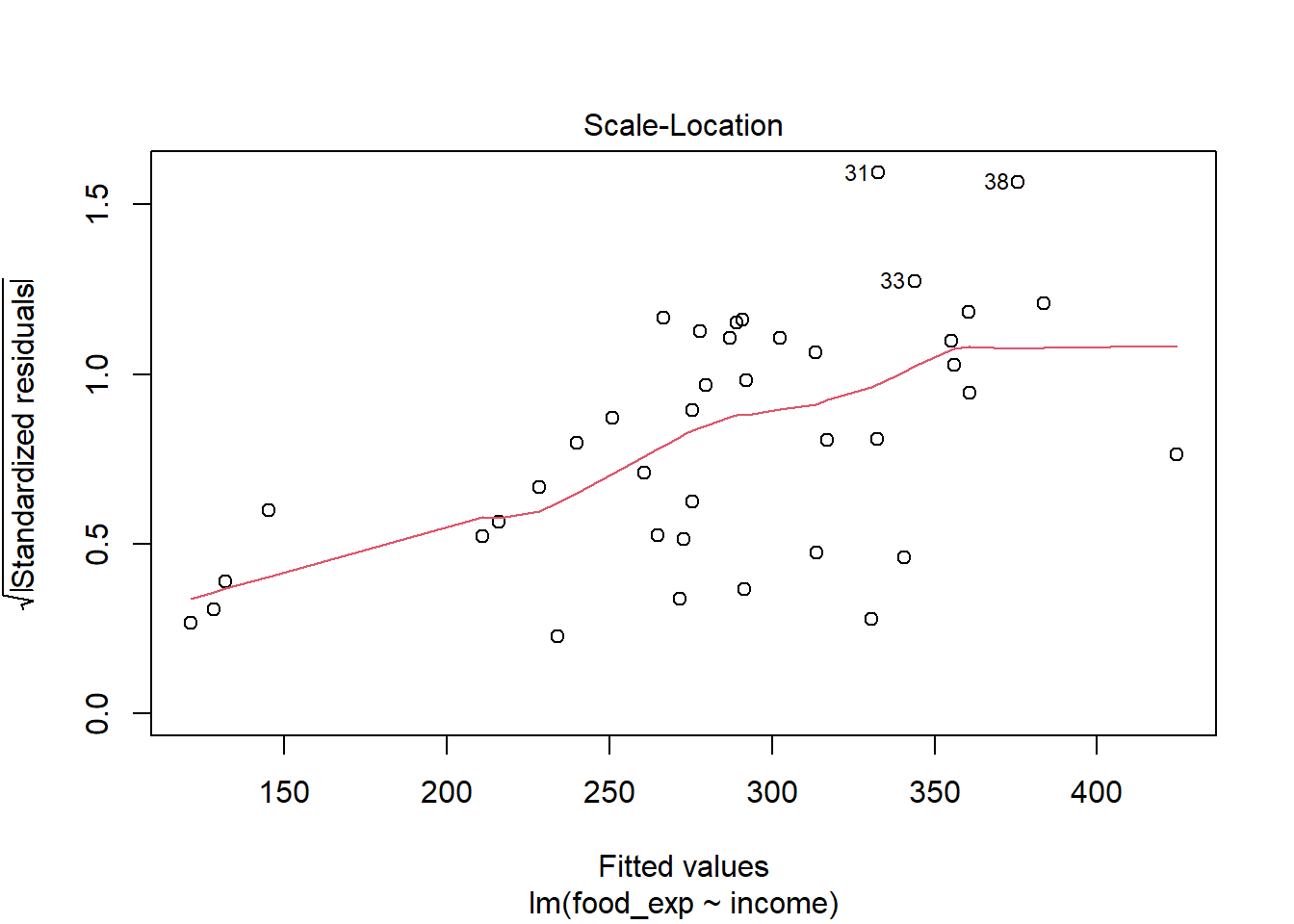
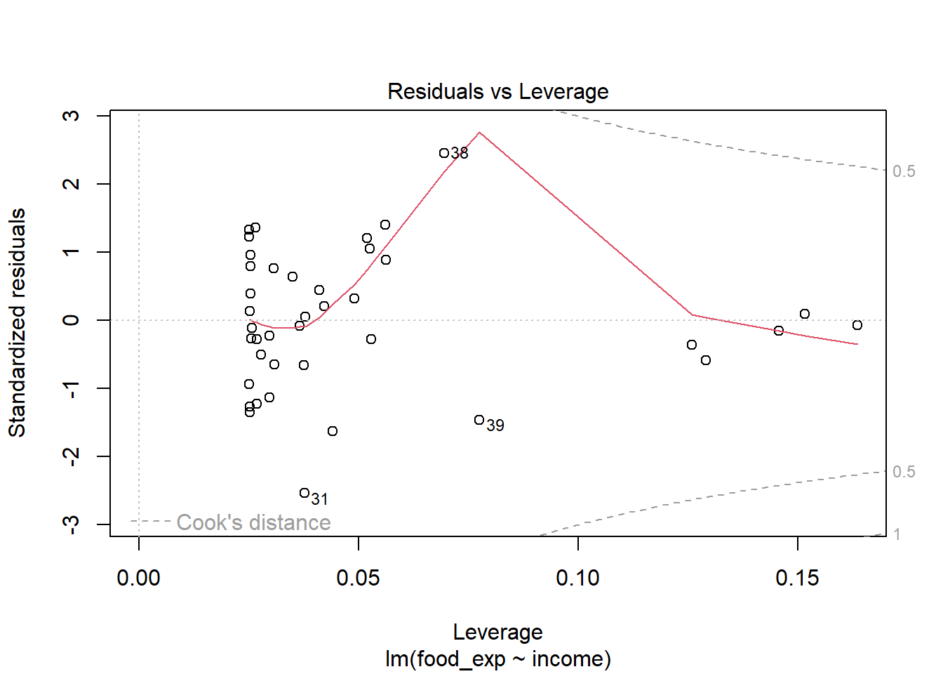
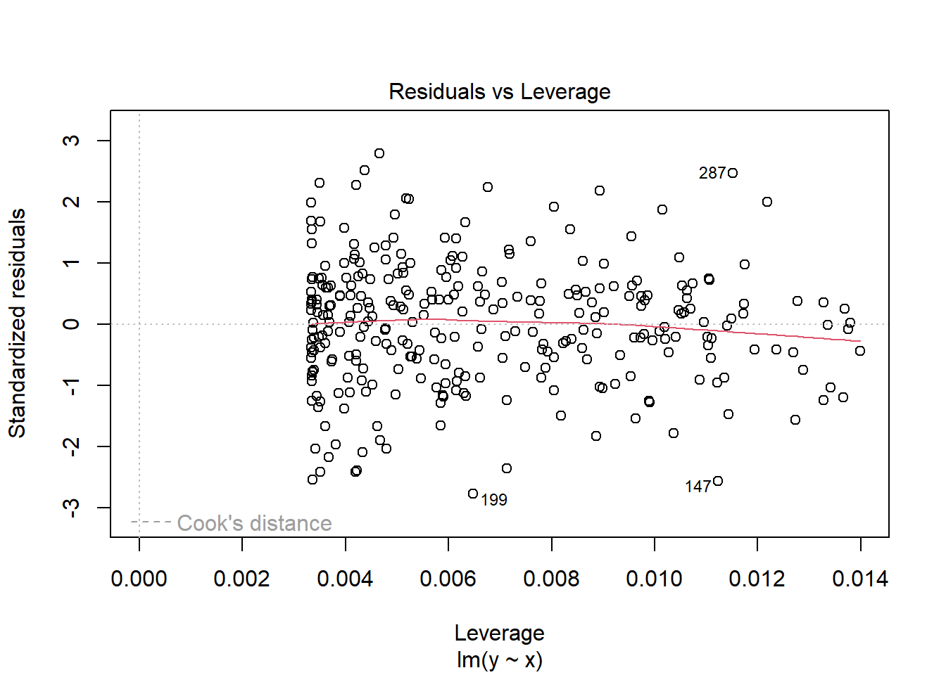
Extras 2: Model dengan Asumsi Homoskedastisitas yang terlanggar

Karena adanya heteroskedastisitas membuat kesalahan standar kuadrat terkecil menjadi keliru, maka diperlukan metode lain untuk menghitung Regresi.

Show the code

library(car)
foodeq <- lm(food_exp~income,data=food)
kable(tidy(foodeq),caption="Regular standard errors in the 'food' equation")

Regular standard errors in the ‘food’ equation
term	estimate	std.error	statistic	p.value
(Intercept)	83.41600	43.410163	1.921578	0.0621824
income	10.20964	2.093263	4.877381	0.0000195

Show the code

cov1 <- hccm(foodeq, type="hc1") #needs package 'car'
food.HC1 <- coeftest(foodeq, vcov.=cov1)
kable(tidy(food.HC1),caption="Robust (HC1) standard errors in the 'food' equation")

Robust (HC1) standard errors in the ‘food’ equation
term	estimate	std.error	statistic	p.value
(Intercept)	83.41600	27.463748	3.037313	0.0042989
income	10.20964	1.809077	5.643566	0.0000018

Show the code

w <- 1/food$income
food.wls <- lm(food_exp~income, weights=w, data=food)
vcvfoodeq <- coeftest(foodeq, vcov.=cov1)
kable(tidy(foodeq), 
  caption="OLS estimates for the 'food' equation")

OLS estimates for the ‘food’ equation
term	estimate	std.error	statistic	p.value
(Intercept)	83.41600	43.410163	1.921578	0.0621824
income	10.20964	2.093263	4.877381	0.0000195

Show the code

kable(tidy(food.wls),
  caption="WLS estimates for the 'food' equation" )

WLS estimates for the ‘food’ equation
term	estimate	std.error	statistic	p.value
(Intercept)	78.68408	23.788722	3.307621	0.0020641
income	10.45101	1.385891	7.541002	0.0000000

Show the code

kable(tidy(vcvfoodeq),caption=
"OLS estimates for the 'food' equation with robust standard errors" )

OLS estimates for the ‘food’ equation with robust standard errors
term	estimate	std.error	statistic	p.value
(Intercept)	83.41600	27.463748	3.037313	0.0042989
income	10.20964	1.809077	5.643566	0.0000018

Show the code

data("food", package="PoEdata")
food.ols <- lm(food_exp~income, data=food)
ehatsq <- resid(food.ols)^2
sighatsq.ols  <- lm(log(ehatsq)~log(income), data=food)
vari <- exp(fitted(sighatsq.ols))
food.fgls <- lm(food_exp~income, weights=1/vari, data=food)

Show the code

stargazer(food.ols, food.HC1, food.wls, food.fgls, type="text",
          column.labels=c("OLS","HC1","WLS","FGLS"),
#          single.row = TRUE, 
#          report = "vc*", 
      header = FALSE,
  dep.var.labels.include = FALSE,
  model.numbers = FALSE,
  dep.var.caption="Dependent variable: 'food expenditure'",
  model.names=FALSE
#          df=FALSE, 
#          digits=2
)


=======================================================================
                               Dependent variable: 'food expenditure'  
                              -----------------------------------------
                                 OLS        HC1       WLS       FGLS   
-----------------------------------------------------------------------
income                        10.210***  10.210*** 10.451*** 10.633*** 
                               (2.093)    (1.809)   (1.386)   (0.972)  
                                                                       
Constant                       83.416*   83.416*** 78.684*** 76.054*** 
                               (43.410)  (27.464)  (23.789)   (9.713)  
                                                                       
-----------------------------------------------------------------------
Observations                      40                  40         40    
R2                              0.385                0.599     0.759   
Adjusted R2                     0.369                0.589     0.753   
Residual Std. Error (df = 38)   89.517              18.750     1.547   
F Statistic (df = 1; 38)      23.789***            56.867*** 119.799***
=======================================================================
Note:                                       *p<0.1; **p<0.05; ***p<0.01

Show the code

stargazer(food.ols, food.HC1, food.wls, food.fgls,
  header=FALSE, 
  title="Comparing various 'food' models",
  type=.stargazertype, # "html" or "latex" (in index.Rmd) 
  keep.stat="n",  # what statistics to print
  omit.table.layout="n",
  star.cutoffs=NA,
  digits=3, 
#  single.row=TRUE,
  intercept.bottom=FALSE, #moves the intercept coef to top
  column.labels=c("OLS","HC1","WLS","FGLS"),
  dep.var.labels.include = FALSE,
  model.numbers = FALSE,
  dep.var.caption="Dependent variable: 'food expenditure'",
  model.names=FALSE,
  star.char=NULL) #supresses the stars

Challenge 2

Lakukan Estimasi Regresi Linear OLS untuk data Pengeluaran Makanan dan Income
Coba untuk melakukan Estimasi Regresi dari Isu/Permasalahan yang ditemukan dari Challenge 1